Draw Circle With Stepper Motor Bresenhams Algorithm

1. Introduction

Straight line drawing is among the important fields of various industries, such equally straight-line interpolation [1], stepper motor cooperative control [2], 3D printing [iii], 3D model edifice [4], and image drawing [5]. To speedily draw directly lines, the speed of the applied algorithm is critical. The Bresenham'due south algorithm [vi,7], DDA algorithm [8,9,x], and midpoint algorithm [xi,12,thirteen] are ii-dimensional straight-line generation algorithms. Amid which, the most famous is the Bresenham'southward algorithm, which is introduced during the 1960s. The advantage of Bresenham'due south algorithm is that all the operations are integers, without division or decimals. This approach is efficient at selecting a gear up of grid points to stand for a straight line in a two-dimensional infinite. Space symmetry and simplifying ciphering are ii major aspects of the algorithm towards high efficiency [14].

Stephenson et al. [15] nowadays a line drawing algorithm based on runs of runs and discussed a number of special cases in the structure of runs and runs; it is proved that the algorithm can also exist practical to curt straight lines; this algorithm is formed to draw the line that has an identical iterative structure to Bresenham's algorithm, except that at each iteration, it is not a pixel that is set but a run of runs; thus, the speed of line cartoon is improved. Li et al. [xvi] proposed a fast line drawing algorithm using round subtraction based on Bresenham'due south algorithm. This algorithm makes use of the respective relationship betwixt the two ends of the line and its symmetry to apace draw multiple pixels, which enhances the speed of drawing direct lines. Liu et al. [1] extended Bresenham's algorithm to a spatial straight line; the straight line is decomposed into the motion of 2 planes, which realize a three-dimensional Bresenham'south algorithm; the actual errors of the algorithm at each sampling point are less than the maximum theoretical error; nevertheless, because of the discriminant containing decimals, the actual line may deviate from the theoretical straight line due to the trouble of retaining decimal digits. Dai et al. [2] also extended Bresenham's algorithm from 2 dimensions to three, and applied information technology to multidimensional stepper motor cooperative control. Although the control accuracy requirements can be met by this algorithm, it is triggered by the interruption of the timer during motion, which leads to a noncontinuous algorithm.

To solve the above problems, a spatial straight line drawing algorithm based on the method of discriminate regions is proposed in this paper. Our innovation is that the discriminant in our algorithm is the integer; only the coordinates of the starting and end bespeak of the spatial straight line are needed to be input in this algorithm; so, the distribution of spatial straight lines in three-dimensional space and the location of the stop point can be quickly adamant, and then the corresponding discriminant is obtained and the selection points of lines in each 3-dimensional mesh are determined. Finally, the selected points are continued to complete the spatial space line drawing. This method tin avoid the decimal in the discriminant completely, so all the operations are integers in the algorithm of this paper; therefore, the trouble of deviation from the theoretical straight line acquired by the retentivity of decimals of pregnant digits will be avoided. This algorithm is applied to the cooperative control of the stepping motor. A proportional integral differential (PID) command algorithm is ofttimes used for the control of a single motor and the parameters demand to be tuned [17]. This paper mainly explains the process of multistep motor cooperative control.

ii. Infinite Line Drawing Algorithm

In this paper, Bresenham's algorithm is extended from a two-dimensional aeroplane to a iii-dimensional space. Meantime, in club to avoid the problem of divergence between the actual direct line and the theoretical straight line caused by the decimals of the discriminant, a method of discriminate regions is designed, and the discriminant is improved.

ii.ane. Analysis of the 2-Dimensional Straight Line of Bresenham'south Algorithm

A recursive step method is used in Bresenham's algorithm [xviii]. The axis with the largest change is taken as the active direction and information technology progresses one grid at a time; the other direction is taken as the passive management, along which whether to progress i grid is decided co-ordinate to the sign of the discriminant, as shown in Effigy 1.

2.2. Assay of the Spatial Straight Line

From the starting to the catastrophe points of the spatial directly line, the deportation of the three axes are generally different, but each axis volition achieve the respective stop coordinates at the same time. The axis with the greatest altitude from the beginning to the end of the directly line is the active direction and progresses a unit of measurement at a fourth dimension; the other two axes are the passive directions and only progress at specific times to maintain their relative slopes (end). The drawing speed and the precision of the direct line are directly determined by where and how long they volition stop [19]. Therefore, the following spatial straight-line cartoon algorithm is designed.

The starting bespeak of spatial direct line is set as

$p_s\left(x_{\mathrm{southward}},y_s,z_s\right),$

and the stop point is

$p_e(x_{\mathrm{due\; east}},y_e,z_e$

), where

$\Delta x=x_e-{\mathrm{ten}}_s$

,

$\Delta y=y_e-y_{\mathrm{due\; south}}$

, and

$\Delta z=z_e-z_s$

. Therefore, the equation for the spatial straight line is:

$$\frac{\mathrm{10}-x_s}{\Delta \mathrm{10}}=\frac{y-y_{\mathrm{due\; south}}}{\Delta y}=\frac{z-z_{\mathrm{due\; south}}}{\Delta z}$$

(1)

Every bit three-dimensional space has intrinsic symmetry [eleven], merely the post-obit types for spatial direct lines in which

$x$

,

$y,$

and

$z$

are all positive directions are discussed. Assume 3-dimensional space consists of innumerable three-dimensional meshes; the side length of each grid is i pixel or ane step angle. In this paper, three-dimensional space is regarded as a cube, and the six surfaces of the cube are, respectively, called: front surface, back surface, left surface, right surface, upper surface, and lower surface; each three-dimensional mesh is chosen a unit grid, the side length of unit grid is chosen a unit, and its length is Fifty, in Figure two.

Figure 2a shows the distribution types of directly lines in iii-dimensional space; assume that the starting point of each straight line is at the origin, and the distribution of the directly line is determined by the end indicate. At that place are vii types, as shown in Figure 2a; by judging the relationship between the values of

$\Delta \mathrm{ten}$

,

$\Delta y$

, and

$\Delta z$

, the position of the end point can be adamant every bit follows:

(1)

If

$\Delta x>\Delta y\ge 0,\Delta x>\Delta z\ge 0$

, the straight line is type ①, as shown in Figure 2a, and the end point is on the right surface of the cube; this type of direct line corresponds to algorithm 1;

$\mathrm{10}$

is taken as the active direction and information technology progresses one filigree at a time;

$\mathrm{y}$

and

$\mathrm{z}$

are taken every bit passive directions, along which whether to progress ane grid is decided according to the sign of the discriminant;

(2)

If

$\Delta \mathrm{10}=\Delta y=\Delta z\ge 0$

, the direct line is blazon ②, as shown in Effigy 2a, and the finish bespeak is on the vertex contrary to the origin; this type of direct line corresponds to algorithm 2;

$\mathrm{x}$

,

$y,$

and

$z$

are taken as the active direction, and progress 1 filigree at a fourth dimension;

(3)

If

$\Delta y>\Delta x\ge 0,\Delta y>\Delta z\ge 0$

, the straight line is type ③, as shown in Figure 2a, and the end bespeak is on the upper surface of the cube; this blazon of direct line corresponds to algorithm 3;

$\mathrm{y}$

is taken equally the agile direction and it progresses one filigree at a time,

$\mathrm{10}$

and

$\mathrm{z}$

are taken as passive directions, along which whether to progress one filigree is decided according to the sign of the discriminant;

(4)

If

$\Delta z>\Delta x\ge 0,\Delta z>\Delta y\ge 0$

, the straight line is type ④, as shown in Figure 2a, and the end bespeak is on the front end surface of the cube; this type of direct line corresponds to algorithm 4;

$\mathrm{z}$

is taken as the active direction and information technology progresses one grid at a time,

$\mathrm{x}$

and

$\mathrm{y}$

are taken as passive directions, along which whether to progress one grid is decided according to the sign of the discriminant;

(5)

If

$\Delta x=\Delta y>\Delta z\ge 0$

, the directly line is type ⑤, every bit shown in Effigy 2a, the end bespeak is on the intersection line of the upper surface and the right surface of the cube; This type of directly line corresponds to algorithm 5;

$\mathrm{10}$

and

$y$

are taken as the active management, and they are progress one grid at a time,

$\mathrm{z}$

is taken as the passive management forth which whether to progress one filigree is decided according to the sign of the discriminant;

(half dozen)

If

$\Delta y=\Delta z>\Delta x\ge 0$

, the straight line is type ⑥, equally shown in Effigy 2a, and the stop point is on the intersection line of the upper surface and the front surface of the cube; this type of direct line corresponds to algorithm 6,

$\mathrm{y}$

and

$z$

are taken equally the agile directions, and they progress one grid at a time;

$\mathrm{ten}$

is taken as the passive direction, along which whether to progress one grid is decided according to the sign of the discriminant;

(7)

If

$\Delta x=\Delta z>\Delta y\ge 0$

, the straight line is type ⑦, equally shown in Figure 2a, and the end signal is on the intersection line of the front end surface and the right surface of the cube; this type of straight line corresponds to algorithm 7;

$\mathrm{10}$

and

$z$

are taken as the active directions, and they progress one grid at a time;

$\mathrm{y}$

is taken equally the passive direction, along which whether to progress one grid is decided according to the sign of the discriminant.

Vii types of straight lines correspond to seven algorithms. By judging the human relationship of

$\Delta x$

,

$\Delta y$

, and

$\Delta z$

, the position of the end of the straight line is adamant, so as to determine the respective algorithm. The flow nautical chart of this algorithm is shown in Figure 3.

ii.three. Method of Discriminate Regions

The basic principle of all the in a higher place algorithms is the same, except for the variable (

$\mathsf{\Delta }x$

,

$\mathsf{\Delta }y$

, and

$\mathsf{\Delta }z$

). The corresponding algorithm is determined by judging the relationship amongst

$\mathsf{\Delta }x$

,

$\mathsf{\Delta }y$

, and

$\mathsf{\Delta }z$

. As an example, this algorithm one is designed and discussed in this paper; and the method of discriminate regions is proposed.

Three-dimensional infinite is divided into innumerable three-dimensional meshes; one of the unit grid is taken, as shown in Figure 4a.

For instance ①, the finish betoken of the straight line is on the correct surface of the cube, so the end indicate of all the straight lines in the unit of measurement filigree is likewise on the correct surface of the unit filigree. Figure 4a shows a directly line in a unit grid, and the coordinate system here is the local coordinate system of each unit grid. Where

${\mathrm{p}}_{\mathrm{i}}$

is the selection point of signal

$i$

, the origin of the

$\left(i+1\right)$

unit filigree, and the starting point of the straight line in the

$\left(i+1\right)$

unit grid.

${\mathrm{p}}_{\mathrm{i}+\mathrm{i}}$

is the intersection of the theoretical directly line and the upper right surface of the unit of measurement grid; considering the option point of

${\mathrm{p}}_{\mathrm{i}+1}$

is an integer point, as shown in Figure 4a, the choice point of

${\mathrm{p}}_{\mathrm{i}+1}$

can only be one of A, B, C, D. Each time a point is selected, it volition serve as the origin of the local coordinate system of the adjacent unit of measurement filigree and the starting point of the line in the next unit grid, where (

$i=0,1,\mathrm{two}\dots \mathrm{due\; north})$

. The correct surface of the unit grid is divided into iv regions (a, b, c, and d) past four lines (e, f, thousand and h); the corresponding selection points of each region are A, B, C, and D, respectively, as shown in Effigy 4b. According to the discriminant, the location of point

${\mathrm{p}}_{\mathrm{i}+1}$

in the region is determined, and the selection point is chosen. The coordinates of the iv points (A, B, C, and D) are, respectively,

$\mathrm{A}\left(x_i+\mathrm{one},y_i+\mathrm{ane},z_i\right)$

,

$\mathrm{B}\left({\mathrm{ten}}_i+\mathrm{i},y_i,z_i\right)$

,

$\mathrm{C}\left({\mathrm{ten}}_i+1,y_i,z_i+1\right),$

and

$\mathrm{D}\left(x_i+1,y_i+1,z_i+\mathrm{ane}\right)$

,where

${\mathrm{d}}_{\mathrm{y}1}$

is the distance between the actual

$\mathrm{y}$

coordinate of point

${\mathrm{p}}_{\mathrm{i}+1}$

and

${\mathrm{y}}_{\mathrm{i}}$

,

${\mathrm{d}}_{\mathrm{y}2}$

is the distance between the actual

$y$

coordinate of point

$p_{i+\mathrm{ane},}$

and

$(y_i+\mathrm{ane})$

,

$d_{z1}$

is the altitude between the actual

$z$

coordinate of betoken

$p_{i+1}$

and

$z_i$

, and

$d_{z2}$

is the distance betwixt the actual

$\mathrm{z}$

coordinate of signal

$p_{i+1}$

and

$\left(z_i+1\right)$

. The

$\mathrm{y}$

and

$\mathrm{z}$

coordinates are determined using Equation (1), as follows:

$$\{\begin{array}{c}y=\frac{\Delta y}{\Delta \mathrm{ten}}\left({\mathrm{10}}_{i+1}-x_s\right)+y_s\\ z=\frac{\Delta z}{\Delta x}\left({\mathrm{ten}}_{i+\mathrm{one}}-{\mathrm{10}}_s\right)+z_{\mathrm{south}}\end{array}$$

(2)

$$\left\{\begin{array}{l}{d}_{y\mathrm{ane}}=y-y_i=\frac{\Delta y}{\Delta x}\left(x_i+\mathrm{one}-x_{\mathrm{southward}}\right)+y_{\mathrm{due\; south}}-y_i\\ d_{y\mathrm{two}}=(y_i+\mathrm{ane})-y=(y_i+1)-\frac{\Delta y}{\Delta x}\left(x_i+\mathrm{ane}-x_s\right)-y_{\mathrm{southward}}\\ d_{z1}=z-z_i=\frac{\Delta z}{\Delta x}\left(x_i+\mathrm{one}-x_s\right)+z_s-z_i\\ d_{z2}=(z_i+\mathrm{i})-z=(z_i+1)-\frac{\Delta z}{\Delta \mathrm{10}}\left(x_i+\mathrm{one}-{\mathrm{10}}_s\right)-z_{\mathrm{south}}\end{array}\right.$$

(three)

$$\{\begin{array}{c}{d}_y=d_{y1}-d_{y2}\\ d_z=d_{z1}-d_{z2}\end{array}$$

(4)

Then, the discriminant is obtained as:

$$\{\begin{array}{c}{d}_y=\mathrm{two}\frac{\Delta y}{\Delta \mathrm{10}}\left({\mathrm{ten}}_i+\mathrm{one}-{\mathrm{ten}}_s\right)-2y_i+2y_s-\mathrm{ane}\\ d_z=\mathrm{ii}\frac{\Delta z}{\Delta \mathrm{ten}}\left(x_i+1-{\mathrm{10}}_s\right)-\mathrm{two}{z}_i+\mathrm{two}{z}_s-1\end{array}$$

(5)

2.4. Improved Discriminant

To simplify the discriminant in Equation (5),

$d_y$

and

$d_z$

beingness all multiplied by

$\Delta x$

; then, an improved discriminant is proposed:

$$\{\begin{array}{c}{\mathrm{Thou}}_i=2\Delta y{\mathrm{ten}}_i-\mathrm{two}\Delta x{y}_i-\mathrm{ii}\Delta y{x}_s+2\Delta \mathrm{ten}{y}_s+2\mathsf{\Delta }\mathrm{y}-\mathsf{\Delta }\mathrm{10}\\ N_i=2\Delta z{x}_i-2\Delta x{z}_i-\mathrm{ii}\Delta z{x}_s+\mathrm{ii}\Delta \mathrm{10}{z}_{\mathrm{south}}+2\mathsf{\Delta }\mathrm{z}-\mathsf{\Delta }\mathrm{x}\end{array}$$

(half dozen)

because

$\Delta \mathrm{10}>0$

,

$G_i$

and

$d_y$

take the same sign, and

$N_i$

and

$d_z$

have the same sign. Therefore, we can decide which point to cull side by side from the signs of

$M_{\mathrm{i}}$

and

${\mathrm{Northward}}_i$

. From Equation (vi), the discriminant at

$i=i+1$

is:

$$\{\begin{array}{c}{M}_{i+1}=2\Delta y{x}_{i+1}-2\Delta x{y}_{i+\mathrm{i}}-2\Delta y{\mathrm{ten}}_{\mathrm{southward}}+\mathrm{two}\Delta x{y}_s+2\mathsf{\Delta }\mathrm{y}-\mathsf{\Delta }\mathrm{x}\\ N_{i+1}=2\Delta z{x}_{i+1}-2\Delta x{z}_{i+\mathrm{i}}-\mathrm{ii}\Delta z{\mathrm{ten}}_s+\mathrm{ii}\Delta x{z}_{\mathrm{due\; south}}+\mathrm{two}\mathsf{\Delta }\mathrm{z}-\mathsf{\Delta }\mathrm{x}\end{array}$$

(seven)

So, the recursive equations are obtained equally:

$$\{\begin{array}{c}{\mathrm{One\; thousand}}_{i+1}={\mathrm{One\; thousand}}_i+2\Delta y-\mathrm{two}\Delta \mathrm{ten}\left(y_{i+\mathrm{i}}-y_i\right)\\ N_{i+\mathrm{one}}={\mathrm{North}}_i+\mathrm{two}\Delta z-\mathrm{ii}\Delta \mathrm{10}\left(z_{i+1}-z_i\right)\end{array}$$

(8)

As the starting point of the spatial direct line is

$p_{\mathrm{due\; south}}\left({\mathrm{ten}}_s,y_s,z_s\right)$

, it is obtained that:

$$\{\begin{array}{c}{\mathrm{10}}_{\mathrm{one}}=x_s\\ y_{\mathrm{i}}=y_{\mathrm{due\; south}}\\ z_1=z_{\mathrm{south}}\end{array}$$

(9)

Considering Equation (6), the initial value of the discriminant is obtained as:

$$\{\begin{array}{c}{\mathrm{Thou}}_1=2\Delta y-\Delta x\\ N_1=\mathrm{two}\Delta z-\Delta \mathrm{ten}\end{array}$$

(10)

ii.5. The Process of Discriminate Region

Considering the positive and negative signs of the above discriminants

${\mathrm{M}}_{\mathrm{i}}$

and

${\mathrm{Northward}}_{\mathrm{i}}$

, which region the indicate

${\mathrm{p}}_{\mathrm{i}+1}$

is in tin exist determined, and then which bespeak of A, B, C, and D will exist selected.

(1)

If

$K_i>0\mathrm{and}{\mathrm{North}}_i<0$

, the signal

$p_{i+\mathrm{ane}}$

is in region a; the point A will be selected at this bespeak.

(ii)

If

$K_i<0\mathrm{and}{N}_i<0$

, the indicate

$p_{i+1}$

is in region b; the point B volition be selected at this point.

(iii)

If

$M_i\langle 0\mathrm{and}{N}_i\rangle 0$

, the betoken

$p_{i+1}$

is in region c; the point C volition exist selected at this point.

(4)

If

$M_i>0\mathrm{and}{\mathrm{Northward}}_i>0$

, the point

$p_{i+1}$

is in region d; the point D will exist selected at this bespeak.

(5)

If

${\mathrm{Yard}}_i=0\mathrm{and}{N}_i<0$

, the point

$p_{i+\mathrm{ane}}$

is on segment e; the point A or B will be selected at this indicate.

(six)

If

$M_i<0\mathrm{and}{N}_i=0$

, the point

$p_{i+\mathrm{i}}$

is on segment f; the point B or C will be selected at this point.

(7)

If

${\mathrm{Thou}}_i=0\mathrm{and}{N}_i>0$

, the point

$p_{i+1}$

is on segment thousand; the point A or D volition be selected at this point.

(eight)

If

${\mathrm{Thou}}_i>0\mathrm{and}{N}_i=0$

, the bespeak

$p_{i+1}$

is on segment h; the point D or A will be selected at this point.

(ix)

If

${\mathrm{Chiliad}}_i=0\mathrm{and}{N}_i=0$

, the point

$p_{i+\mathrm{one}}$

is at fundamental signal o; the point A or B or C or D will be selected at this point.

Therefore, only the signs of

${\mathrm{Thousand}}_i$

and

${\mathrm{North}}_i$

are needed to gauge to make up one's mind the side by side selection point. Bold that north steps are required from the starting point to ending indicate of the spatial straight line, the judging algorithm flow chart is given in Figure 5.

3. Algorithm Verification and Application

3.1. Algorithm Verification Based on Matlab

For the purpose of verification of the algorithm in this paper, it is causeless that the starting point of the spatial straight line is

$p_{\mathrm{due\; south}}\left(0,0,0\right)$

, 300 integers of 0–100 are randomly generated in MATLAB, and three numbers of them are a group of coordinates as the end point of a straight line; There are totally 100 groups, and one grouping of them is taken as an example, such as

$p_e\left(\mathrm{viii},6,\mathrm{five}\right)$

; therefore,

$\mathsf{\Delta }x=8$

,

$\mathsf{\Delta }y=6$

, and

$\mathsf{\Delta }z=5$

.

From Equation (ten), the initial value of the discriminants are

${\mathrm{Thou}}_1=4$

and for

${\mathrm{N}}_1=\mathrm{two}$

. The above algorithm is used to draw the spatial directly lines, as shown in Effigy 6.

In this case study, the terminate point coordinate for the

$\mathrm{ten}$

-axis is viii, which required eight steps forward. Thus, the

$x$

-centrality progressed one unit of measurement at a time, and the bodily x-axis value coincided with the theoretical value. The terminate points for the

$y$

and

$z$

-axis are 6 and 5, respectively. Therefore, there are two steps without progression forth the

$y$

-axis, and there are three forth the

$z$

-centrality. In Effigy 6a,

${\mathsf{\delta }}_i$

is the fault of each stride, and n steps needed totally for the straight-line, and then:

$${\delta }_i=\sqrt{\varphi x_i{}^2+\varphi y_i{}^{\mathrm{two}}+\varphi z_i{}^{\mathrm{ii}}},\left(i=1,2\dots n\right)$$

(eleven)

In Figure 6b, the blackness dashed line is the actual generated spatial direct line, and the reddish dashed line is the theoretical Spatial straight line. The cylinder is the minimum inclusive region of the spatial directly-line straightness mistake [20], which is parallel to the theoretical direct line. All parts of the spatial direct line fatigued by the algorithm are in the cylinder, whose diameter is the maximum error of the spatial directly line [21,22], and

$\delta =\mathrm{thou}a\mathrm{ten}({\delta }_i)$

, all the results are shown in Effigy 7.

Effigy 7a–c, respectively, bear witness the largest change of x-axis, y-axis, and z-centrality in 100 groups of data and the local enlarged cartoon, and B is the enlarged effigy of A, where the blackness line is the x-axis, red line is the y-centrality, and bluish line is the z-axis.

iii.ii. Error Analysis

When the point

$p_{i+1}$

is at the center O of the right surface of the unit of measurement grid, the altitude from

$p_{i+1}$

to whatever point of A, B, C, and D is the same

$({\delta }_t)$

, which is chosen the maximum theoretical mistake of the spatial straight line, equally shown in Figure 8.

Co-ordinate to Figure 8, the maximum theoretical mistake

${\delta }_t=0.7071\ast \mathrm{50}$

. Where L is the side length of the unit grid, that is, the step length of each step of each centrality—for example, in general industrial machine tools—50 represents the moving distance of the actuator driven by a pulse of stepping motor. The stride angle of the stepping motor is θ, subdivided is s; the pulse number of one plough of the stepping motor is

$p_m$

; and the screw pitch is p, then:

The stepper motor receives one pulse, and the lead screw movement distance L is

If

$\theta =\mathrm{one.8}°$

,

$\mathrm{south}=\mathrm{two}$

,

$P=2\mathrm{mm}$

, obtain:

$\mathrm{50}=5\ast {\mathrm{ten}}^{-\mathrm{iii}}\mathrm{mm}$

, and the maximum theoretical fault

${\delta }_t=3.54\ast {10}^{-\mathrm{iii}}\mathrm{mm}.$

It tin be seen that the value of L is related to the parameters of the stepping motor and the actuator, and the fault distribution of each straight line is every bit shown in Figure 9.

Let L be 1, and in Effigy nine,

${\delta }_{M\mathrm{due\; east}an}$

is the average value of error of each straight line in 100 straight lines; this reflects the concentration trend of fault of each straight line.

${\delta }_{\left(Mean-Kax\right)}$

is the maximum value of

${\delta }_{\mathrm{Grand}ean},$

which is 0.4119; here, the straight-line error is relatively big.

${\delta }_{\left(\mathrm{Thou}ean-\mathrm{1000}i\mathrm{due\; north}\right)}$

is the minimum value of

${\delta }_{Mea\mathrm{north}}$

, which is 0.2469; hither, the straight-line error is relatively minor.

${\delta }_{\left(Mea\mathrm{northward}-M\mathrm{eastward}an\right)}$

is the average value of

${\delta }_{Mean},$

which is 0.3792; this reflects the concentration trend of errors of all straight lines.

${\delta }_{Max}$

is the maximum fault of each directly line in 100 direct lines, that is, the straightness error.

${\delta }_{\left(Max-Ma\mathrm{10}\right)}$

is the maximum value of

${\delta }_{Max},$

which is 0.7071; hither, the straightness error is relatively large.

${\delta }_{\left(\mathrm{One\; thousand}ax-\mathrm{Chiliad}in\right)}$

is the minimum value of

${\delta }_{Max},$

which is 0.7071; hither, the straightness error is relatively small-scale.

${\delta }_{\left(Max-M\mathrm{east}an\right)}$

is the boilerplate value of

${\delta }_{Kax,}$

which is 0.6472; this reflects the concentration trend of the straightness error of the straight line.

${\delta }_{\mathrm{South}td}$

is the standard deviation of the error of each direct line in 100 directly lines; this reflects the measures of dispersion of each direct-line fault.

${\delta }_{\left(Std-\mathrm{Chiliad}ax\right)}$

is the maximum value of

${\mathsf{\delta }}_{\mathrm{Std}},$

which is 0.2250; hither, the measures of dispersion are relatively big.

${\delta }_{\left(\mathrm{Due\; south}td-\mathrm{Chiliad}in\right)}$

is the maximum value of

${\mathsf{\delta }}_{\mathrm{Std},}$

which is 0.1390; here, the measures of dispersion are relatively pocket-size.

${\delta }_{\left(Std-\mathrm{Yard}ea\mathrm{northward}\right)}$

is the boilerplate value of

${\delta }_{\mathrm{Southward}td,}$

which is 0.1534; this reflects the concentration trend of the measures of dispersion of all straight-line errors.

From the in a higher place results, all errors are less than or equal to the maximum theoretical error of 0.7071.

In addition, according to the algorithm provided by Liu [i], a random function in MATLAB to set several sets of samples including origin and target points is used. So, Liu'due south algorithm and our algorithm are all programmed in MATLAB to generate a direct line with the above-mentioned randomly generated origin and terminate points. In this fashion, the ideal line is drawn, and the actual line generated by these two different algorithms are obtained, respectively. Finally, the ideal curve and the actual curve generated past the 2 algorithms are fatigued in i graph, as shown in Figure 10 (green and blue lines represent the results of retaining four and one decimal places, respectively, and the detailed explanation of Figure 10a is in the sixth paragraph of the fourth section).

A specific example is now given to explain the difference. As Liu's paper shows: given that the 2 stop-points of a directly-line segment are specified at positions (0, 0, 0) and (10, 7, half-dozen), it follows that k_yx = 0.7, and yard_zx = 0.vi, then

ε(y _one) = y _i − y _0r − 0.5 = g_yx − 0.five = 0.2

(14)

ε(z _i) = z ₁ − z _0r − 0.5 = m_zx − 0.5 = 0.1

(15)

From the above 2 equations, information technology is possible to summate the generated pixels and the decision parameters at each inter 10 position, starting from 0, 0, 0, as listed in Table ane. The mistake listed in the final column of the table is the distance between the generated pixel and the given line path at each inter x position.

Bringing this example into the algorithm in this article can obtain the information in Table 2.

In addition, the departure between the 7th and 9th steps of the two methods tin can be clearly seen below in Table 1, Tabular array 2, and Figure 11. When pace 9 is performed, the error is dissimilar, which can be seen from Table 1 and Table 2, respectively, and the mistake is sightly less than that in the literature.

3.3. Conversion of Unit of measurement Filigree Number and Pulse Number

Step motor is an open-loop command motor which transforms electrical pulse signal into angular deportation or linear displacement [23]. When a pulse is received, it will bulldoze the step motor to rotate a stock-still angle (step angle θ) according to the gear up management. The algorithm in this paper can be used for controlling three stepping motors cooperatively. In the research of Dulf [24,25] et al., a new method for designing a fractional-order controller and a method for designing a DC motor speed control fractional-gild PI controller are proposed, and the method is proved through an example assay. The feasibility and superiority of the fractional-social club controller can greatly reduce the overshoot and make its performance amend than the traditional Kessler controller. Through specific experiments, its operation is evaluated and compared to other types of implementation possibilities. Three stepper motors command the

$x$

-axis,

$y$

-centrality, and

$z$

-axis, respectively; the three-dimensional space described in the algorithm is the working space of three stepping motors; and the unit is a pulse.

$\mathsf{\Delta }\mathrm{x}$

,

$\mathsf{\Delta }\mathrm{y},$

and

$\mathsf{\Delta }\mathrm{z}$

are the number of pulses required to accomplish the target point for the

$x$

motor,

$y$

motor, and

$z$

motor, respectively. The number of forward steps mentioned in this paper is the number of pulses required for the centrality with the largest moving distance.

In industrial machine tools, the three coordinate axes are all driven by lead screw, and the atomic number 82 screw pitch is

$P$

mm. Three axes are set to movement

$x$

mm,

$y$

mm,

$z$

mm, respectively; then, the footstep motor turns a circle while lead spiral moves

$P$

mm(one pitch), and three motors rotate

$\frac{x}{P}$

circumvolve,

$\frac{y}{P}$

circle, and

$\frac{z}{P}$

circle, respectively, to reach the target point. The step angle

$\theta$

of all three stepper motors is 1.viii°, and the subdivision

$s$

is eight. Co-ordinate to Equation (12), 1600 pulses are needed for ane turn of the stepper motor. The number of pulses of the three stepper motors for reaching the target point are (1600 ×

$\frac{x}{P}$

), (1600 ×

$\frac{y}{P}$

), (1600 ×

$\frac{z}{P}$

), respectively.

3.4. Algorithm Extension

The algorithm in this paper can be extended to v dimensions; assuming that the other two axes are A and B, respectively, the respective discriminant is H and M, respectively. According to Equation (8), the H and K are obtained:

$$\{\begin{array}{c}{H}_{i+\mathrm{one}}=H_i+2\Delta A-2\Delta x\left(A_{i+1}-A_i\right)\\ {\mathrm{Thousand}}_{i+\mathrm{i}}=K_i+2\Delta B-\mathrm{ii}\Delta x\left(B_{i+\mathrm{ane}}-B_i\right)\end{array}$$

(16)

Considering Equation (10), the initial value of the discriminant H and K are obtained as:

$$\{\begin{array}{c}{H}_1=2\Delta A-\Delta x\\ K_{\mathrm{one}}=\mathrm{ii}\Delta B-\Delta x\end{array}$$

(17)

According to the above rules, when

$H_{i+1}>0$

,

$A_{i+1}=A_i+1$

, and when

${\mathrm{Grand}}_{i+1}>0$

,

$B_{i+1}=B_i+\mathrm{i}$

. Therefore, the algorithm in this newspaper tin can exist extended to 5 or more than dimensions, which means that more motors tin be controlled cooperatively by this algorithm in this paper.

4. Word

Matlab Simulation Discussion

The type ① is discussed as 1 example of the algorithm in this paper; that is, the cease signal of the directly line is on the right surface of the cube, and algorithm 1 is designed. The 10 axis is taken as the agile direction, and progresses i unit at a time; y and z are taken every bit the passive direction; by judging the sign of discriminant

${\mathrm{Thou}}_i$

and

${\mathrm{Northward}}_i$

, which regions of the right surface of the unit grid the point is located in volition exist determined, and so whether or not to progress one unit of measurement will be determined. At that place are seven types of spatial line distribution; for the other six types, the finish position of the direct line is different, and the variables (

$\mathsf{\Delta }\mathrm{ten}$

,

$\mathsf{\Delta }y$

, and

$\mathsf{\Delta }z$

) are different, just the algorithm structure is the same: simply the corresponding variables need to be exchanged. In improver, in this paper, the

$\mathsf{\Delta }\mathrm{x}$

,

$\mathsf{\Delta }\mathrm{y}$

, and

$\mathsf{\Delta }\mathrm{z}$

in the discriminant of the algorithm possess a proportion relation. For example, if

$\mathsf{\Delta }x=8000$

,

$\mathsf{\Delta }y=6000$

, and

$\Delta z=5000$

, the corresponding step size of 8000, and there is the greatest common gene (

$C_f$

), that is m, then

$\Delta x^{\ast }=\frac{\Delta x}{C_f}=8$

,

$\Delta y^{\ast }=\frac{\Delta y}{C_f}=\mathrm{six}$

, and

$\Delta z^{\ast }=\frac{\Delta z}{C_f}=5$

; the

$\Delta x^{\ast }$

,

$\Delta y^{\ast }$

, and

$\Delta z^{\ast }$

are taken every bit variables of discriminants; moreover, the discriminants are all integers. Therefore, the proposed algorithm could be simplified to calculate for drawing spatial direct lines. The 100 groups of data are randomly generated by MATLAB, and the algorithm is verified in this newspaper. It is proved that the algorithm is suitable for straight lines in any direction.

According to the algorithm verification results in Department 3, several sets of data generated by MATLAB are brought into the iii-dimensional algorithm of Liu [one], and the results are shown in Figure 12.

It can exist seen from the results of the comparing algorithm that this algorithm produced the aforementioned results as the algorithm in this newspaper; meanwhile, the same example is brought into Dai [2], in which besides the same results occurred. It is noted that the selection points for the

$y$

and

$z$

-centrality in the comparison algorithm are judged separately in the XY and XZ planes. In addition, the discriminant contains decimals in the reference algorithm; all the same, there are not the higher up two phenomena in the algorithm of this paper.

Because of the retention number of significant digits and the gradual accumulation of the discriminant the positive and negative signs of the discriminant may exist inverse, the selective betoken also may be altered. Furthermore, at that place is a greater divergence of the drawn straight line from the theoretical directly line, which increases the straightness mistake. In order to verify the possibility of the above issues, the discriminant of unlike decimal places (four, 3, ii, and one decimals) is calculated past the comparison algorithm, after testing; when the discriminant retains ane decimal, the direct line volition deviate from its ideal straight line, as shown in Figure 10a.

In the Effigy 10a, B is enlarged pictures of A; the blackness and red lines represent the

$x$

and

$y$

-axis, respectively; greenish and blue lines correspond the results of retaining 4 and ane decimal places, respectively. It can be seen in the figure that the z-centrality deviates from the theoretical directly line with the reserved one decimal place: at this time, the straightness error

$\delta$

is greater than the maximum theoretical error of 0.7071. The z-axis oscillates on the theoretical direct line with the reserved four decimal places.

Additionally, the post-obit conclusions have been reached through multiple verifications; the Liu [i] algorithm will not deviate from the theoretical line when more than two decimals are reserved, and may deviate from the theoretical line when one decimal is reserved.

In this newspaper, according to a given rule (such as a pixel or a step bending), three-dimensional space is divided into innumerable iii-dimensional meshes, namely unit of measurement grids. The right surface of each unit filigree is divided into iv regions, and two discriminants are determined at the aforementioned fourth dimension to make up one's mind the selection point. One point is selected each fourth dimension: this betoken would be the origin of the coordinate organisation of the next unit of measurement grid, and also the starting point of the straight line in this unit of measurement grid. The discriminants of the algorithm in this paper are all integers; that the problem of deviation from the theoretical straight line caused by the retention of decimals of significant digits can be avoided. Some other literatures also proposed some new algorithms or related fault analysis: they verify the effectiveness and advantages of the algorithm through comparison and analysis with other related literatures [26,27]. In this article, the effectiveness and advantages of our algorithm are shown through MATLAB simulation, comparing, and assay with other related literature. In that location are still some shortcomings in this algorithm. A big number of samples are needed for comparative analysis to verify whether the computational efficiency of this algorithm is improved; now, this algorithm is only suitable for the space straight line, and not for the space curve.

five. Conclusions

First, the Bresenham's algorithm is extended to three-dimensional space in this paper. Bresenham algorithm is 2-dimensional. To depict three-dimensional infinite directly lines, a novelty method of discriminate regions is proposed in this paper. Based on the discriminant, the selection points for each step will be provided. Merely the coordinates of the starting and catastrophe points of the spatial direct line are needed to exist input in this algorithm, and the discriminants of the region tin exist rapidly determined. All the discriminants are integers, making the calculations unproblematic to quickly draw the spatial straight line; and the problem of deviation from the theoretical straight line caused by the retention of decimals of significant digits can exist avoided. By analyzing the error of the straight line, the event shows that the error of the algorithm is related to the step length

$\mathrm{L}$

. The maximum theoretical error is

$\frac{\sqrt{\mathrm{two}}}{\mathrm{two}}\times \mathrm{Fifty}$

, where

$\mathrm{L}=\mathrm{P}/{\mathrm{p}}_m$

. In addition, in this paper, the

$\mathsf{\Delta }\mathrm{x}$

,

$\mathsf{\Delta }\mathrm{y}$

, and

$\mathsf{\Delta }\mathrm{z}$

in the discriminant of the algorithm possess a proportion relation, which could be replaced by the simplest integer. Moreover, the discriminants of this newspaper are all integers; therefore, the proposed algorithm in this paper could be used to calculate drawing both short and long straight lines more simply than the algorithm of decimals of other discriminants, while the accurateness is guaranteed. Meanwhile, the algorithm'due south conversion application between unit of measurement grid number of algorithm and pulse of motors is performed, and the algorithm in this paper can be used for decision-making three stepper motors cooperatively or exist extended to 5 dimensions.

Author Contributions

Conceptualization, J.W.; methodology, S.X.; software, J.Y.; validation, S.X., J.Y.; formal analysis, Due south.X.; investigation, J.W., Y.L.; resources, Y.Fifty.; information curation, S.Ten.; writing—original draft preparation, South.X.; writing—review and editing, P.B.; visualization, T.Southward.; supervision, Y.L., T.Southward.; project assistants, Y.L.; funding acquisition, J.W. All authors have read and agreed to the published version of the manuscript.

Funding

This investigation is supported by the National Natural Science Foundation of China (31370999). (Information for disclosures can be taken from the online abstract system after entering all authors).

Conflicts of Involvement

The authors declare no conflict of interest.

References

1. Liu, X.Due west.; Cheng, K. Three-dimensional extension of Bresenham's algorithm and its application in direct-line interpolation. Proc. Inst. Mech. Eng. Part B J. Eng. Manuf. 2002, 216, 459–463. [Google Scholar]
2. Dai, Yard.; Chen, Y.; Zheng, C.; Yiming, G. Design of multistep stepper motor coordinated control system based on bresenham algorithm. In Proceedings of the 2017 24th International Briefing on Mechatronics and Motorcar Vision in Practice (M2VIP), Auckland, New Zealand, 21–23 November 2017. [Google Scholar]
3. Chen, Z.; Shen, Z.; Guo, J.; Cao, J.; Zeng, X. Line drawing for 3D printing. Comput. Graph. 2017, 66, 85–92. [Google Scholar]
4. Meng, Q.; Geng, Thou.; Zhang, J. A line drawing method of the 3D models based on fractional sharpening. In Proceedings of the 2012 International Briefing on Image Assay and Signal Processing, Zhejiang, Red china, 9–11 November 2012; pp. nine–11. [Google Scholar]
5. Guo, T.; Wang, Y.; Zhou, Y.; He, Z.; Tang, Z. Geometric object 3D reconstruction from single line drawing image with Lesser-Up and Top-Downwards classification and sketch generation. In Proceedings of the 2017 14th IAPR International Conference on Certificate Analysis and Recognition (ICDAR), Kyoto, Japan, ix–xv November 2017; pp. 670–676. [Google Scholar]
6. Skala, V. An intersecting modification to the bresenham algorithm. Comput. Graph. Forum 1987, half-dozen, 343–347. [Google Scholar]
7. Bresenham, J.East. Algorithm for computer control of a digital plotter. IBM Syst. J. 1965, four, 25–thirty. [Google Scholar]
8. Nguyen, D.T. A rotation method for binary document images using DDA algorithm. ACM Symp. Doc. Eng. 2008, 267–270. [Google Scholar] [CrossRef]
9. Govil-Pai, Southward. Principles of Figurer Graphics: Theory and Practice Using OpenGL and Maya, 1st ed.; Springer: Berlin/Heidelberg, Germany, 2010. [Google Scholar]
10. Cieśliński, J.Fifty.; Moroz, L.V.; Walczyk, C.J. Fast exact digital differential analyzer for circle generation. Appl. Math. Comput. 2015, 271, 68–79. [Google Scholar]
11. Lau, W.-C.; Erramilli, A.; Wang, J.; Willinger, W. Self-like traffic generation: The random midpoint displacement algorithm and its backdrop. In Proceedings of the IEEE International Conference on Communications, Seattle, WA, Us, 6 August 2002. [Google Scholar]
12. Jilesen, J.; Kuo, J.; Lien, F.-S. Three-dimensional midpoint displacement algorithm for the generation of fractal porous media. Comput. Geosci. 2012, 46, 164–173. [Google Scholar]
13. Garcia-Falset, J.; Marino, G.; Zaccone, R. An explicit midpoint algorithm in Banach spaces. J. Nonlinear Convex Anal. 2017, 18, 1933–1952. [Google Scholar]
14. Au, C.; Woo, T. Three dimensional extension of Bresenham's Algorithm with Voronoi diagram. Comput. Des. 2011, 43, 417–426. [Google Scholar]
15. Stephenson, P.; Litow, B. Running the line: Line drawing using runs and runs of runs. Comput. Graph. 2001, 25, 681–690. [Google Scholar]
16. Li, X.; Shao, X. Fast line drawing algorithm by circular subtraction based on Bresenham. In Proceedings of the SPIE—The International Gild for Optical Applied science, Bellingham, WA, U.s., 13 January 2012; Volume 8349, p. xx. [Google Scholar]
17. Muresan, C.; Copot, C.; Birs, I.; De Keyser, R.; Vanlanduit, S.; Ionescu, C.Thousand. Experimental Validation of a Novel Auto-Tuning Method for a Partial Order PI Controller on an UR10 Robot. Algorithms 2018, 11, 95. [Google Scholar] [CrossRef]
18. Pitteway, M.L.Five.; Watkinson, D.J. Bresenham'south algorithm with Grayness calibration. Commun. ACM 1980, 23, 625–626. [Google Scholar] [CrossRef]
19. Labatut, V. Continuous average straightness in spatial graphs. J. Circuitous Netw. 2017, half-dozen, 269–296. [Google Scholar] [CrossRef]
20. Zhang, Q.; Fan, Yard.-C.; Li, Z. Evaluation method for spatial straightness errors based on minimum zone condition. Precis. Eng. 1999, 23, 264–272. [Google Scholar] [CrossRef]
21. Endrias, D.H.; Feng, H.-Y.; Ma, J.; Wang, L.; Abu Taher, M. A combinatorial optimization approach for evaluating minimum-zone spatial straightness errors. Measurement 2012, 45, 1170–1179. [Google Scholar] [CrossRef]
22. Wen, X.; Song, A. An improved genetic algorithm for planar and spatial straightness error evaluation. Int. J. Mach. Tools Manuf. 2003, 43, 1157–1162. [Google Scholar] [CrossRef]
23. Li, J.; Meng, D. Dynamic and Adjustable New Blueprint Four-Vector SVPWM Algorithm for Application in a Five-Phase Induction Motor. Energies 2020, 13, 1856. [Google Scholar] [CrossRef]
24. Dulf, E.-H.; Susca, M.; Kovács, L. Novel Optimum Magnitude Based Fractional Order Controller Design Method. IFAC-PapersOnLine 2018, 51, 912–917. [Google Scholar] [CrossRef]
25. Muresan, C.I.; Folea, S.; Mois, G.; Dulf, Eastward. Development and implementation of an FPGA based fractional order controller for a DC motor. Mechatronics 2013, 23, 798–804. [Google Scholar] [CrossRef]
26. Hassan, T.-U.; Abbassi, R.; Jerbi, H.; Mehmood, Grand.; Tahir, Chiliad.F.; Cheema, Chiliad.M.; Elavarasan, R.Yard.; Ali, F.; Khan, I. A Novel Algorithm for MPPT of an Isolated PV System Using Push Pull Converter with Fuzzy Logic Controller. Energies 2020, 13, 4007. [Google Scholar] [CrossRef]
27. Du, L.; Ma, Q.; Ben, J.; Wang, R.; Li, J. Duality and Dimensionality Reduction Discrete Line Generation Algorithm for a Triangular Filigree. ISPRS Int. J. Geo-Inf. 2018, 7, 391. [Google Scholar] [CrossRef]

Figure i. Schematic of Bresenham'south algorithm. Note: (

$x_{i+\mathrm{i}}-x_i)>\left(y_{i+1}-y_i\right)$

, and so

$\mathrm{x}$

is the active direction,

$\mathrm{y}$

is passive direction.

Figure i. Schematic of Bresenham'due south algorithm. Notation: (

$x_{i+\mathrm{one}}-x_i)>\left(y_{i+1}-y_i\right)$

, so

$\mathrm{10}$

is the active direction,

$\mathrm{y}$

is passive direction.

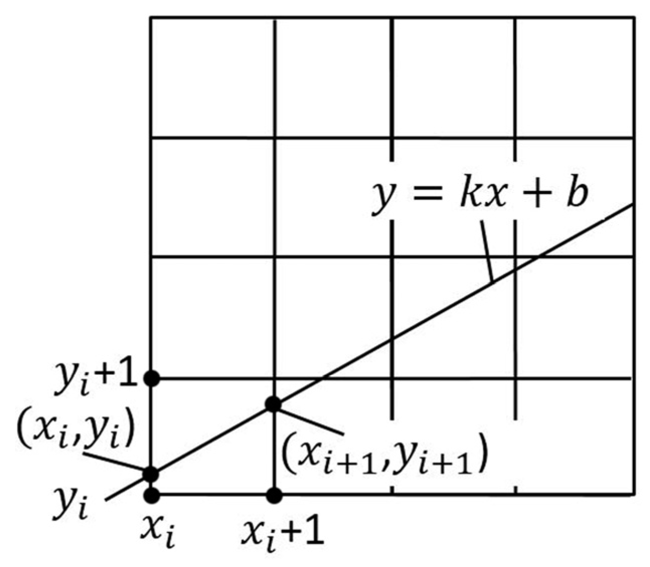
Figure 2. 3-dimensional infinite. (a) Distribution types of straight lines in three-dimensional infinite. (b) Three-dimensional space meshing.

Figure 2. Three-dimensional space. (a) Distribution types of straight lines in iii-dimensional infinite. (b) Three-dimensional space meshing.

Effigy 3. Catamenia chart for judging the distribution of straight lines in three-dimensional infinite.

Effigy 3. Flow chart for judging the distribution of direct lines in 3-dimensional space.

Effigy iv. Method of discriminate regions. (a) A straight line in a unit of measurement grid. (b) The position of the desire signal in the aeroplane.

Figure 4. Method of discriminate regions. (a) A direct line in a unit filigree. (b) The position of the desire point in the plane.

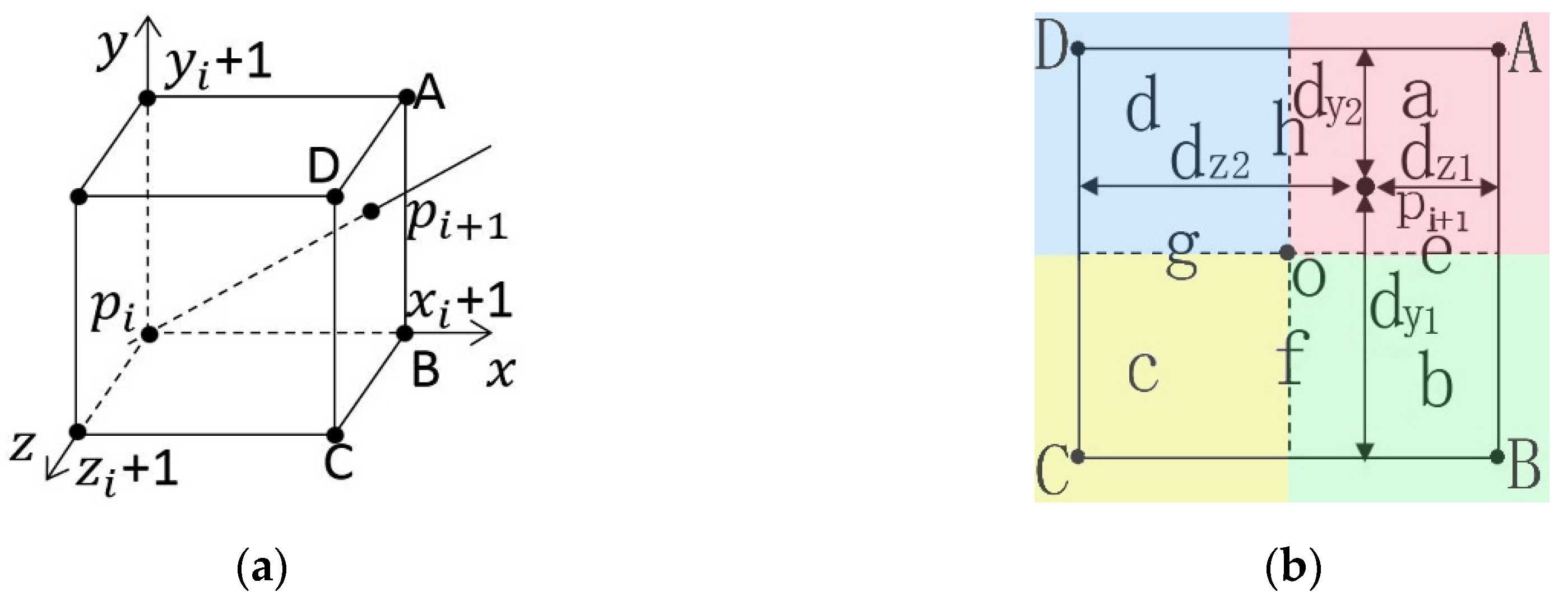
Figure 5. The judging algorithm catamenia chart for determining the side by side point.

Figure 5. The judging algorithm flow chart for determining the next bespeak.

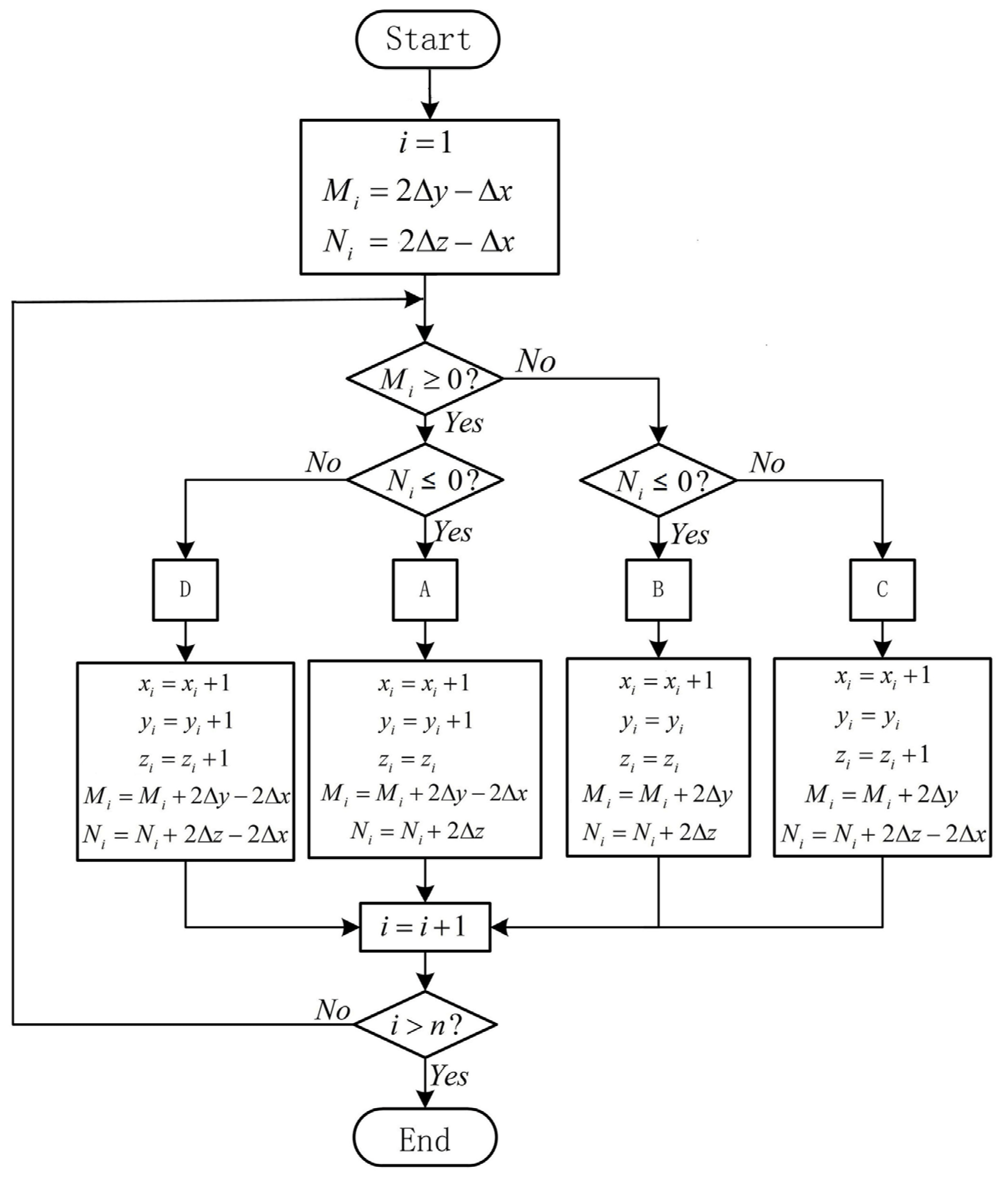
Figure 6. Results of the spatial straight-line algorithm. (a) The motion procedure of each axis. (b) Spatial directly line and straightness fault. Annotation: Figure 6a shows the motion procedure for each axis. The ordinate is the number of units, and the abscissa is the number of forward steps. The black, reddish, and blue lines represent the

$x$

,

$y,$

and

$z$

-axis. The solid line is the theoretical value, while the dashed line is the actual value.

Figure half dozen. Results of the spatial straight-line algorithm. (a) The motion procedure of each centrality. (b) Spatial straight line and straightness fault. Note: Figure 6a shows the move process for each axis. The ordinate is the number of units, and the abscissa is the number of forrad steps. The black, red, and blue lines represent the

$x$

,

$y,$

and

$z$

-axis. The solid line is the theoretical value, while the dashed line is the actual value.

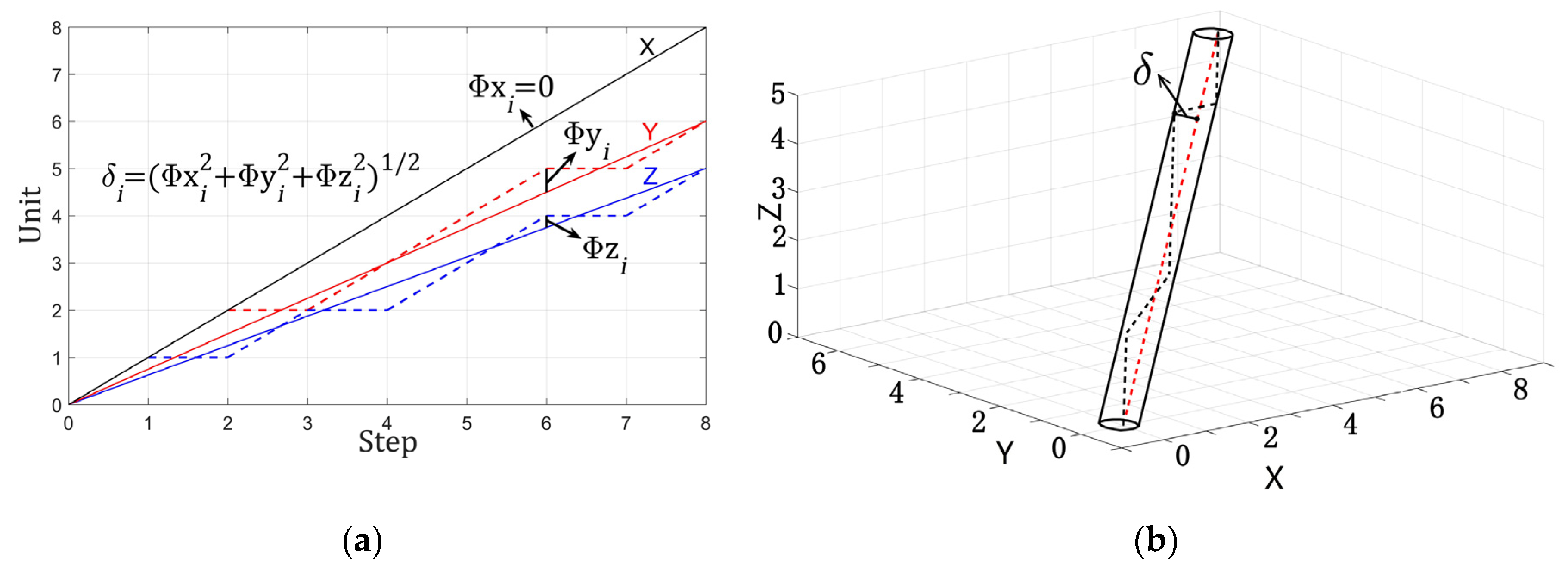
Figure vii. The 100 groups of straight-line results. (a) The

$\mathrm{x}$

-centrality with the largest change. (b) The

$\mathrm{y}$

-axis with the largest change. (c) The

$\mathrm{z}$

-axis with the largest modify.

Effigy seven. The 100 groups of straight-line results. (a) The

$\mathrm{x}$

-centrality with the largest change. (b) The

$\mathrm{y}$

-centrality with the largest modify. (c) The

$\mathrm{z}$

-axis with the largest modify.

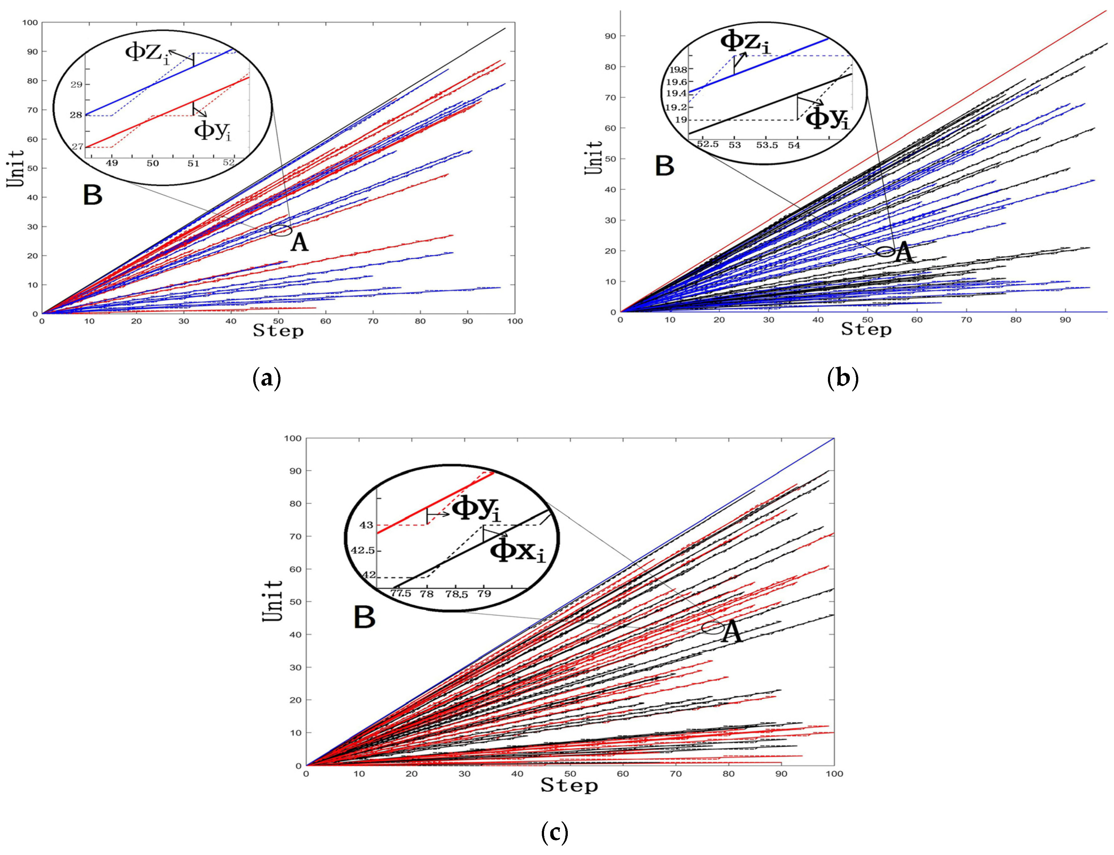
Figure 8. The maximum theoretical error of a spatial straight line. (a) A directly line in a unit grid. (b) The position of the maximum theoretical mistake signal in the plane.

Figure 8. The maximum theoretical error of a spatial direct line. (a) A straight line in a unit grid. (b) The position of the maximum theoretical error point in the airplane.

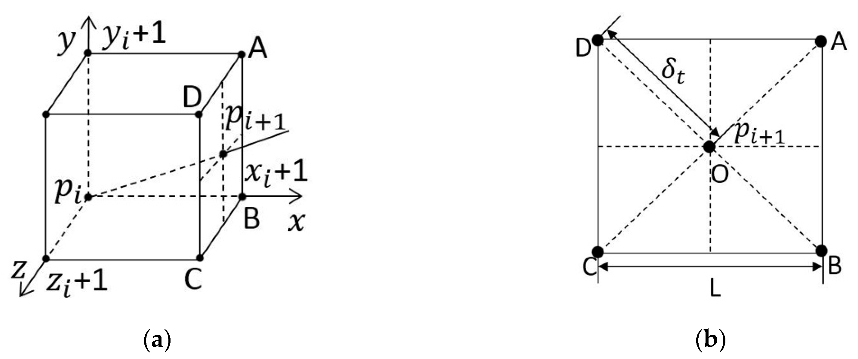
Figure 9. The error distribution.

Figure ix. The error distribution.

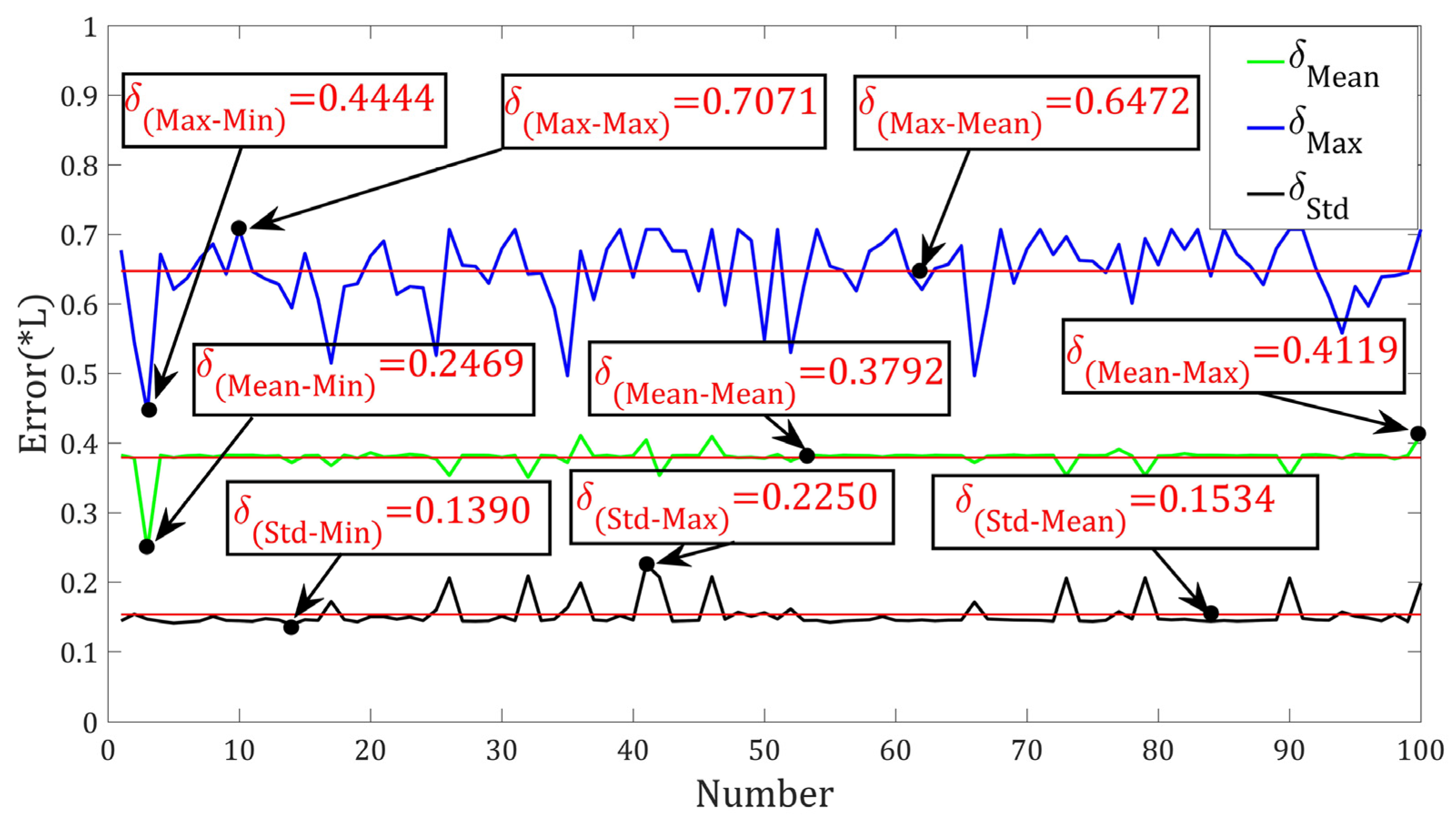
Figure 10. The event of algorithm to generate straight lines. (a) Liu's algorithm keeps one decimal place. (b) Algorithm in this article.

Effigy ten. The result of algorithm to generate direct lines. (a) Liu'southward algorithm keeps one decimal identify. (b) Algorithm in this article.

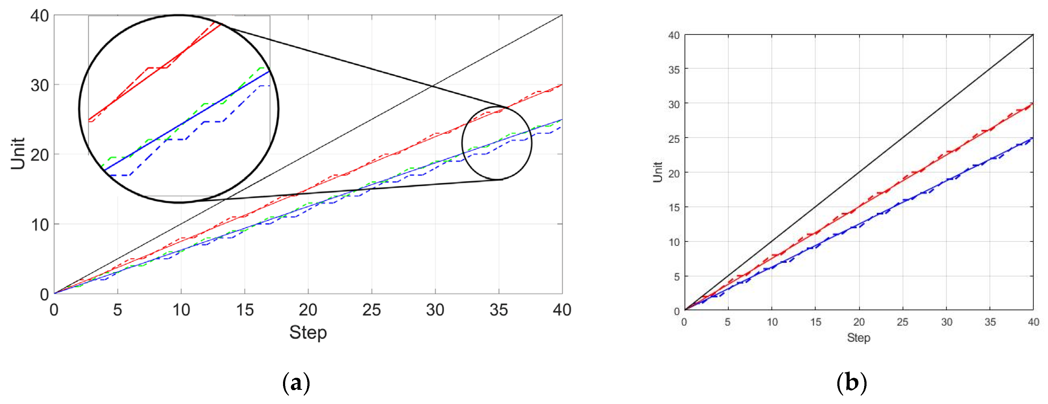
Figure 11. Differences between two different algorithms. (a) Line generation based on Liu's algorithm (b) Line generation based on this commodity's algorithm.

Effigy eleven. Differences between two different algorithms. (a) Line generation based on Liu'southward algorithm (b) Line generation based on this commodity'southward algorithm.

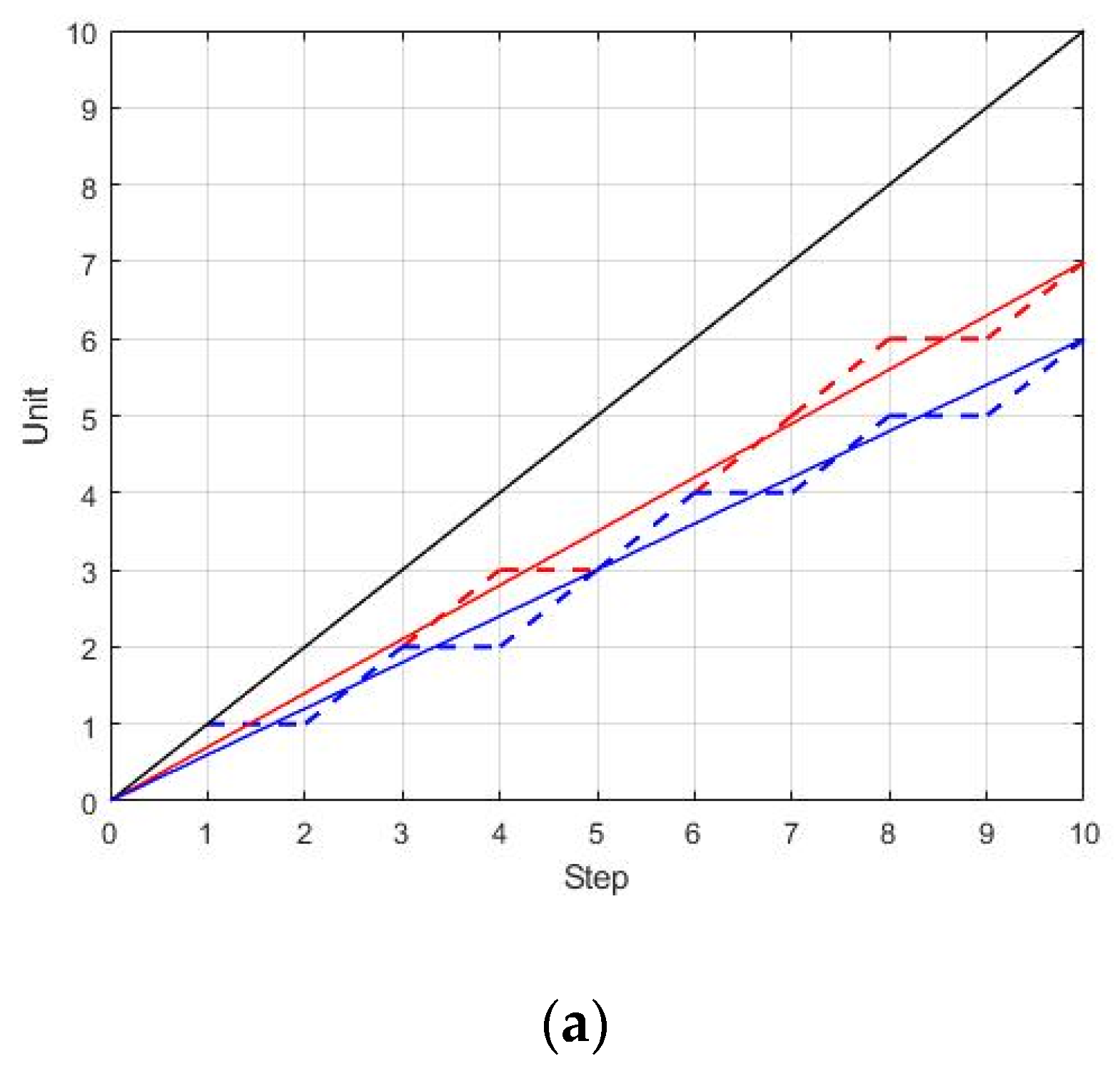
Figure 12. Results of the spatial straight-line algorithm. (a) The movement process of each axis. (b) Spatial straight line and straightness fault.

Figure 12. Results of the spatial direct-line algorithm. (a) The move process of each centrality. (b) Spatial directly line and straightness error.

Tabular array i. Line generation based on Liu's algorithm.

Tabular array i. Line generation based on Liu'south algorithm.

i	xi	yir	zir	ε(y i+1)	ε(z i+1)	Mistake
0	0	0	0	0.2	0.ane	0
one	1	one	ane	−0.one	−0.3	0.374887
ii	2	1	ane	0.6	0.3	0.336918
3	3	2	ii	0.3	−0.one	0.220564
4	4	3	two	0	0.5	0.441129
5	five	4	3	−0.3	0.1	0.428700
6	6	4	4	0.4	−0.3	0.441129
7	7	5	4	0.ane	0.3	0.225064
8	viii	half-dozen	5	−0.2	0.1	0.336918
9	9	six	5	0.5	0.v	0.374887
10	10	7	6	0.2	0.ane	0

Table 2. Line generation based on this article's algorithm.

Table 2. Line generation based on this commodity's algorithm.

i	teni	yi	zi	Mi	Northwardi	Error
0	0	0	0	0	0	0
one	1	one	1	iv	ii	0.374887
2	two	1	1	−2	−6	0.336918
3	3	2	2	12	half-dozen	0.220564
four	4	3	2	six	−ii	0.441129
5	5	4	3	0	xviii	0.428700
6	6	4	4	−6	10	0.441129
seven	7	5	5	8	2	0.220564
viii	8	vi	five	2	−6	0.336918
9	9	half-dozen	6	−4	half-dozen	0.334534
x	10	7	six	ten	−ii	0

© 2020 by the authors. Licensee MDPI, Basel, Switzerland. This commodity is an open access article distributed nether the terms and atmospheric condition of the Artistic Commons Attribution (CC BY) license (http://creativecommons.org/licenses/by/4.0/).

schermerhornsaffive.blogspot.com

Source: https://www.mdpi.com/1996-1073/13/19/5002/htm

Share this post